Simplex Method

What have we learned so far?

  LP的标准形式（原始问题）

\[\text{(LP)} \quad \begin{aligned} \text{min} \quad & \mathbf{c}^T \mathbf{x} \\ \text{s.t.} \quad & \mathbf{Ax} = \mathbf{b} \\ & \mathbf{x} \ge 0 . \end{aligned}\]

1. 如果它的可行域\(P\)非空，那么它至少有一个vertex（extreme point）。——from Resolution Theorem
2. 如果\(P\)非空且目标值 \(\mathbf{z}\)不是无界的，那么最优值在\(P\)的（至少）一个顶点（极值点）处取到。——from Fundamental Theorem
3. 可行域\(P\)只有有限个顶点（极值点）。——\(C(n,m)\)
4. Vertices可以用代数的方法来生成，和bfs的一样。

Implications

• 当\(C(n,m)\)很小时，可以枚举出所有的bfs's（vertices）来找到最优的那个作为最优解。——Enumerate Method
• 当\(C(n,m)\)变大时，我们需要一个更系统的、有效的方法来做这个工作。——Simplex Method

3.1 Simplex Method

  Convinced by Prof. George B. Dantzig in 1947.

3.1.1 Basic ideas

Phase 1:

• Step 1 (Starting)
    找到一个初始的extreme point (ep) 或声明\(P\)是空的。

Phase 2：

• Step 2 (Checking optimality)
    如果当前ep是最优的，STOP！
• Step 3 (Pivoting)
    Move to a better ep.
    Return to Step 2.

从Step 3回到Step 2的过程称为一次iteration。
  如果我们不重复同一个ep，那么算法将总是在有限次迭代后终止。—— a finite algorithm
  如何有效地生成更好的极值点？—— basic feasible solutions

What else have we learned?

• 可行域\(P\)中一点\(\mathbf{x}\)为极值点，当且仅当\(\mathbf{x}\)是关于某个基\(\mathbf{B}\)的一个basic feasible solution。
• 最多存在\(C(n,m)\)个基本可行解。当\(\text{rank}(A) = m \le n\)，那么一个bfs可以通过\(\mathbf{A} = \begin{bmatrix} \mathbf{B} & \mathbf{N}\end{bmatrix} \ \mathbf{x} = \begin{bmatrix} \mathbf{x}_B \\ \mathbf{x}_N \end{bmatrix}\)并且令\(\mathbf{x}_N = 0\)以解出\(\mathbf{x}_B = \mathbf{B^{-1} b}\)。

Challenge:
  当我们从一个bfs移动到另一个时，我们真的移动了吗？
  如果没有的话，我们可能陷入循环了！

3.1.2 Nondegeneracy

例

\[\begin{cases} & x_1 + x_2 \le 40 \\ & 2x_1 + x_2 \le 60 \\ & x_1 \le 20 \\ & x_1 ,\ x_2 \ge 0 \end{cases} \quad \Leftrightarrow \quad \begin{cases} & x_1 + x_2 + s_1 = 40 \\ & 2x_1 + x_2 + s_2 = 60 \\ & x_1 + s_3 = 20 \\ & x_1 ,\ x_2 ,\ s_1 ,\ s_2 ,\ s_3 \ge 0 \\ \end{cases}\]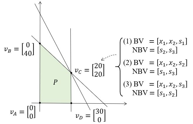

Observations:

• 如果一个ep是由正好有\(m\)个正的basic variables和\(n-m\)个为零的non-basic variables组成的，那么两者之间应该是一一对应的。——a nondegenerate bfs
• 只有当basic variables中至少有一个为零时，这个ep才可能与不止一个bfs对应。——a degenerate bfs

Terminology: 如果所有的bfs都是非退化的，那么LP nondegenerate。

Property 1: 如果一个bfs \(\mathbf{x}\)是非退化的，那么\(\color{blue}{\mathbf{x}}\)由n个hyperplane唯一确定。

Why? \(n\) hyperlanes? Where are they?
  \(\mathbf{A} = \begin{bmatrix}\mathbf{B} & \mathbf{N}\end{bmatrix}\)，\(\mathbf{x} = \begin{bmatrix}\mathbf{x_B} \\ \mathbf{x_N}\end{bmatrix} = \begin{bmatrix}\mathbf{B^{-1}b} \\ 0\end{bmatrix}\)，令\(\mathbf{M} = \begin{bmatrix}\mathbf{B} & \mathbf{N} \\ 0 & \mathbf{I} \end{bmatrix}\)，那么\(\mathbf{M}\)是非奇异的，并且\(\mathbf{Mx} = \begin{bmatrix}\mathbf{B} & \mathbf{N} \\ 0 & \mathbf{I} \end{bmatrix} \begin{bmatrix}\mathbf{x_B} \\ \mathbf{x_N}\end{bmatrix} = \begin{bmatrix}\mathbf{b} \\ 0\end{bmatrix}\)。因此，\(\mathbf{x} = \begin{bmatrix}\mathbf{x_B} \\ \mathbf{x_N}\end{bmatrix} = \mathbf{M}^{-1} \begin{bmatrix}\mathbf{b} \\ 0\end{bmatrix}\)由\(n\)个线性无关的hyperpalne唯一决定。

  \(\mathbf{M}^{-1}\)（或\(\mathbf{M}\)）是LP的fundamental matrix，\(\mathbf{M}^{-1} = \begin{bmatrix}\mathbf{B}^{-1} & -\mathbf{B}^{-1}\mathbf{N} \\ 0 & \mathbf{I} \end{bmatrix}\)。因此，若\(\mathbf{B}^{-1}\)已知即可得到\(\mathbf{M}^{-1}\)。

Property 2: 如果一个bfs \(\mathbf{x}\)是退化的，那么\(\color{blue}{\mathbf{x}}\)由超过n个hyperplane超定。

  因为除了\(\begin{bmatrix}\mathbf{B} & \mathbf{N} \\ 0 & \mathbf{I} \end{bmatrix} \begin{bmatrix}\mathbf{x_B} \\ \mathbf{x_N}\end{bmatrix} = \begin{bmatrix}\mathbf{b} \\ 0\end{bmatrix}\)的\(n\)个hyperplane外，还至少有一个basic variable \(\mathbf{x}_i = 0\)（因为bfs是退化的），也是一个hyperplane。

Property 3: 对于一个退化的有\(p(\lg m)\)个正的元素的bfs \(\mathbf{x}\)，可能有\(\left(\begin{matrix}n-p \\ n-m \end{matrix}\right) = \frac{(n-p)!}{(n-m)!(m-p)!}\)个不同的bfs与同一个极值点相关。

3.2 Simplex Method under Nondegeneracy

Basic idea: 利用a simple pivoting scheme从一个bfs(ep)移动到另一个bfs(ep)。

• 只考虑neighboring bfs(ep)，而非同时考虑所有bfs(ep)。

Definition: 如果两个bfs有\(\color{green}{m-1}\)个共同的basic variable（不是指它们的值），那么这两个bfs adjacent。

Observations:

• 在非退化的情况下，每个基本可行解（极值点）都有\(n-m\)个adjacent neighbors。
• 对于一个bfs，所有的相邻bfs都可以通过将一个非基本变量从零增加到正的并且将一个基本变量从正的减小为零来到达。——Pivoting

3.2.1 Pivoting

  一个nonbasic变量进入basis（从0到positive），同时一个basic变量离开basis（从positive到0）。

Who and where are my neighbours?
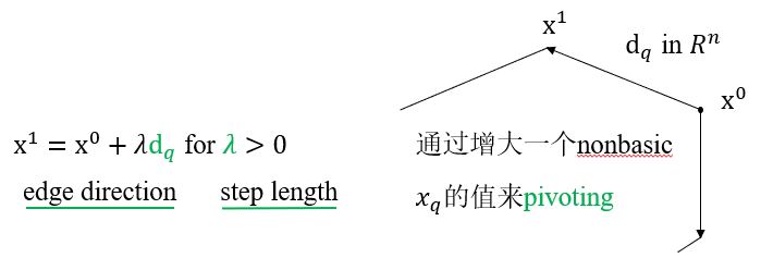
  当前的ep沿着\(P\)的boundary edge走到相邻ep。当前ep有\(n-m\)个邻居，应有\(n-m\)条edge directions指向相邻的极值点，与各个非基变量（n.b.v.）的增加相对应。令edge direction \(\mathbf{d}_q \in \mathbf{R}^n\)与非基变量\(x_q\)的增加相对应。

Where are these edge directions?

3.2.2 Edge direction

Conjecture: \(\mathbf{d}_q\)是\(\mathbf{M}^{-1}\)中与\(x_q\)相关的列，i.e. \(\color{green}{\mathbf{d}_q= \begin{bmatrix} - \mathbf{B}^{-1} \mathbf{A}_q & 0 & \cdots & 0 & 1 & 0 & \cdots & 0\end{bmatrix}^T }\) 。其中，\(\mathbf{A} = \begin{bmatrix}\mathbf{A}_1 & \mathbf{A}_2 & \cdots & \mathbf{A}_n \end{bmatrix}\)。

例

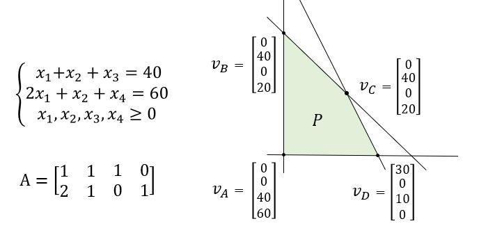
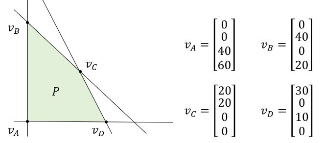
在\(v_A\)处，basic variables为\(\{x_3,x_4\}\)，nonbasic variables为\(\{x_1,x_2\}\)，
所以\(\mathbf{B}=\begin{bmatrix} 1 & 0 \\ 0 & 1 \end{bmatrix}\)，\(\mathbf{N}=\begin{bmatrix} 1 & 1 \\ 2 & 1 \end{bmatrix}\)，\(\mathbf{M}^{-1} = \begin{bmatrix} 1 & 0 & -1 & -1 \\ 0 & 1 & -2 & -1 \\ 0 & 0 & 1 & 0 \\ 0 & 0 & 0 & 1 \end{bmatrix}\)

General case: 对于\(\lambda \ge 0\)，

\[\mathbf{x}(\lambda) = \mathbf{x} + \lambda \mathbf{d}_q = \begin{bmatrix} \mathbf{x_B} \\ \mathbf{x_N} \end{bmatrix} + \lambda \begin{bmatrix} -\mathbf{B}^{-1} \mathbf{A}_q \\ 0 \\ \vdots \\ 1 \\ \vdots \\ 0 \end{bmatrix}\]

（1）非基变量，均为0，除了\(x_q\)被\(\lambda\)增大，i.e. \(\mathbf{x_N}(\lambda) = \mathbf{x_N} + \lambda \begin{bmatrix} 0 & \cdots & 1 & \cdots & 0 \end{bmatrix}^T\)
（2）基变量，由于\(\mathbf{Bx_B + Nx_N = b}\)，因此\(\mathbf{x_B = B^{-1}b - B^{-1}Nx_N}\)。当\(x_q\)被\(\lambda\)增大时，其它的非基变量仍为0，那么\(\mathbf{x_B}(\lambda) = \mathbf{B^{-1}b} - \lambda \mathbf{B}^{-1} \mathbf{A}_q\)。因此，\(\mathbf{d}_q= \begin{bmatrix}- \mathbf{B}^{-1} \mathbf{A}_q \\ \mathbf{e}_q \end{bmatrix}\)。

问： edge direction \(\mathbf{d}_q\)总是可行的方向吗？这要求对于足够小的步长\(\lambda \gt 0\)，需要满足\(\mathbf{x}(\lambda) = \mathbf{x} + \lambda \mathbf{d}_q \in P\)。即必须有\(\mathbf{Ax}(\lambda) = \mathbf{b}\)且\(\mathbf{x}(\lambda) \ge 0\)。等同于要证\(\mathbf{Ad}_q = 0\)且\(\mathbf{x}(\lambda) \ge 0\)。

—Yes，当问题是非退化的时候，每个edge direction都是一个可行的方向。

证：（1）由\(\mathbf{MM}^-1 = \mathbf{I}\)可得\(\mathbf{Ad}_q = 0\)；
  （2）对于非退化的情况，\(\mathbf{x}(\lambda) = \mathbf{x} + \lambda \begin{bmatrix}- \mathbf{B}^{-1} \mathbf{A}_q \\ \mathbf{e}_q \end{bmatrix}\)。因此，当\(\lambda\)足够小时\(\mathbf{x}(\lambda) \ge 0\)。i.e. 在非退化的情况下，an edge direction \(\mathbf{d}_q\) is a feasible direction!

—No，当问题是退化的时候，不一定每个edge direction都是一个可行的方向。

3.2.3 Reduced cost

问：如果当前bfs不是最优的，那么哪个相邻的bfs是更好的呢？也就是说，要往哪个edge direction移动呢？或者说，哪个非基变量是一个好的转入候选呢？

Observations:

\[\begin{aligned} \mathbf{z}(\mathbf{x}(\lambda)) & = \mathbf{c }^T \mathbf{x}(\lambda) \\ & = \mathbf{c }^T (\mathbf{x} + \lambda \mathbf{d}_q) \\ & = \mathbf{z}(\mathbf{x}) + \lambda \begin{bmatrix} \mathbf{c }_B^T & \mathbf{c }_N^T \end{bmatrix} \begin{bmatrix} -\mathbf{B}^{-1} \mathbf{A}_q \\ \mathbf{e}_q \end{bmatrix} \\ & = \mathbf{z}(\mathbf{x}) + \lambda (\mathbf{c}_q - \mathbf{c }_B^T \mathbf{B}^{-1} \mathbf{A}_q) \\ & = \mathbf{z}(\mathbf{x}) + \lambda r_q \end{aligned}\]

如果\(r_q = \mathbf{c}^T \mathbf{d}_q = c_q - \mathbf{c }_B^T \mathbf{B}^{-1} \mathbf{A}_q) \lt 0\)，那么\(\mathbf{d}_q\)是一个好的方向。

Definition: \(\color{green}{r_q = \mathbf{c}^T \mathbf{d}_q = c_q - \mathbf{c }_B^T \mathbf{B}^{-1} \mathbf{A}_q}\)称为关于变量\(\mathbf{x}_q\)的reduced cost。

Theorem: 如果\(\mathbf{x} = \begin{bmatrix} \mathbf{B}^{-1} \mathbf{b} \\ 0 \end{bmatrix}\)是与\(\mathbf{B}\)有关的一个bfs，并且对于某些n.b.v. \(x_q\)有\(r_q \lt 0\)，那么\(\mathbf{d}_q = \begin{bmatrix}-\mathbf{B}^{-1} \mathbf{A}_q \\ \mathbf{e}_q \end{bmatrix} \in \mathbf{R}^n\)会带来更好的目标值。

Observations:

• 对于一个基本变量\(x_q \in \mathbf{B}\)，\(r_q =\mathbf{c}_q - \mathbf{c}_B^T \mathbf{B}^{-1} \mathbf{A}_q = \mathbf{c}_q - \mathbf{c}_q = 0\)。
• 任意满足\(r_q \lt 0\)的\(\mathbf{d}_q \ (x_q \text{ n.b.v.})\)将被用于单纯形法。减小最多的方向为\(\min_{j: \text{nonbasic}} \{ \frac{\mathbf{c}^T \mathbf{d}_j}{\parallel \mathbf{d}_j \parallel} \}\)，但对于单纯形法而言，贪心策略是无效的，因为无法预知再下一步会减小多少。

3.2.4 Optimality check by reduced cost

问：如果对于任意的n.b.v. \(x_q\)，\(r_q \ge 0\)，当前基本可行解是最优的吗？

Theorem: 给定一个基为\(\mathbf{B}\)的bfs \(\mathbf{x} = \begin{bmatrix} \mathbf{B^{-1} b} \\ 0 \end{bmatrix}\)，如果\(\color{green}{r_q \ge 0 , \forall \text{ n.b.v. } x_q}\)，那么\(\color{green}{\mathbf{x}}\)是最优的。

证：思路为证明\(\mathbf{c}^T \mathbf{y} \ge \mathbf{c}^T \mathbf{x}^0 \ge 0 ,\ \forall \mathbf{y} \in P\)，即证明\(\mathbf{c}^T(\mathbf{y} - \mathbf{x}^0) \ge 0\)。

问：该定理反过来还成立吗？i.e. "如果一个bfs \(\mathbf{x}\)是最优的，那么\(r_q \ge 0 , \forall \text{ n.b.v. } x_q\)"
答：仅在非退化的情况下成立。因为在退化的情况下，在向其它方向移动的时候，可能会移动到可行域外面。

最优解的唯一性

corollary 1: 如果对于所有的n.b.v. \(x_q\)都有reduced cost \(r_q \gt 0\)，那么bfs \(\mathbf{x}\)是唯一的最优解。
corollary 2: 如果\(\mathbf{x}\)是一个有些\(r_{q_1}, r_{q_2}, \ldots, r_{q_k} = 0\)的最优bfs，那么\(P\)中任意满足\(\mathbf{y} = \mathbf{x} + \sum_{i=1}^k {y_{q_i} d_{q_i}}\)也是最优的。

3.2.5 Step length

  已知顶点\(\mathbf{x}\)，移动后的点为\(\mathbf{x}(\alpha) = \mathbf{x} + \alpha \mathbf{d}_q ,\ \alpha \gt 0\)，那么需要移动多远才能使得\(\mathbf{x}(\alpha)\)是一个相邻的bfs呢？

  已知\(\mathbf{x}(\alpha) = \mathbf{x} + \alpha \mathbf{d}_q ,\ \alpha \gt 0\)，且\(r_q = \mathbf{c}^T \mathbf{d}_q = c_q - \mathbf{c }_B^T \mathbf{B}^{-1} \mathbf{A}_q \lt 0\)。由\(\mathbf{A d}_q = 0\)可得\(\mathbf{A x}(\alpha) = \mathbf{Ax = b}\)。

Case 1：如果\(\mathbf{d}_q \ge 0\)，那么\(\mathbf{x}(\alpha) \ge 0 ,\ \forall \alpha \ge 0\)。因此\(\mathbf{x}(\alpha) \in P ,\ \forall \alpha \ge 0\)并且当\(\alpha \rightarrow + \infty\)时，\(\mathbf{c}^T \mathbf{x}(\alpha) = \mathbf{c}^T \mathbf{x} + \alpha \mathbf{c}^T \mathbf{d}_q \rightarrow - \infty\)。也就是说，如果沿着某个每个元素都大于0的方向\(\mathbf{d}_q\)移动时reduced cost是负的，那么就一直沿这个方向走向无穷，目标函数值会一直减小且解不会到可行域外。

Theorem: 对于某个n.b.v. \(x_q\)，如果\(\mathbf{x}\)是一个满足\(\mathbf{d}_q \ge 0\)且\(r_q \lt 0\)的bfs，那么这个LP是无界的。

Case 2：\(\mathbf{d}_q\)中至少有一个元素\(\lt 0\)。为了保证\(\mathbf{x}(\alpha) \ge 0\)，我们需要令\(\alpha = \min_{i : \text{basic}} \{\frac{x_i}{-d_{qi}} \vert d_{qi} \lt 0\}\)，其中\(\color{green}{\min_{i : \text{basic}} \{\frac{x_i}{-d_{qi}} \vert d_{qi} \lt 0\}}\)为minimal ratio test。

Note 1：\(-d_{qi} \lt 0\)只能发生在基变量上（\(x_i \in \mathbf{B}\)）。
Note 2：\(\alpha\)是由minimum ratio test决定的。
Note 3：在非退化的情况下，对于b.v. \(x_i\)有\(x_i \gt 0\)，可以推出\(\alpha \gt 0\)，进而有\(\mathbf{x}(\alpha)\)是另一个极值点。
    对于退化的bfs，有可能\(x_i = 0\)，\(\alpha = 0\)，所以\(\mathbf{x}(\alpha)\)还停在同一个极值点处。

Theorem: \(\mathbf{x}\)是一个bfs，如果step length \(\alpha\)是由minimum ratio test决定的，那么\(\mathbf{x}(\alpha) = \mathbf{x} + \alpha \mathbf{d}_q\)是一个相邻的bfs。

  注意，当bfs \(\mathbf{x}\)是非退化的时，\(\mathbf{x}(\alpha)\)会移动到相邻的极值点处。

3.2.6 Summary

单纯形法的关键步骤：

• Step 1 找到一个与\(\mathbf{A = [B \vert N]}\)对应的bfs \(\mathbf{x}\)。
• Step 2 检查n.b.v.的\(r_q = \mathbf{c}^T \mathbf{d}_q (= c_q - \mathbf{c }_B^T \mathbf{B}^{-1} \mathbf{A}_q)\)
   如果\(r_q \ge 0 ,\ \forall \text{ nonbasic } x_q\)，那么当前的bfs是最优的；
   否则，选择一个\(r_q \lt 0\)，进行下一步。
• Step 3 如果\(\mathbf{d}_q \ge 0\)，那么LP是unbounded；
   否则，找到\(\alpha = \min_{i : \text{basic}} \{\frac{x_i}{-d_{qi}} \vert -d_{qi} \lt 0\}\)，那么\(\mathbf{x} \leftarrow \mathbf{x} + \alpha \mathbf{d}_q\)是一个新的bfs，更新\(\mathbf{B}\)和\(\mathbf{N}\)，返回Step 2。

Theorem: 在非退化假设下，单纯形法在有限次数的迭代后终止，得到无界最小值或给定LP的最优解。

3.2 Two-Phase Method

• Step 1 令右侧向量非负：
  \(\text{(LP)} \quad \begin{aligned} \text{min} \quad & \mathbf{c}^T \mathbf{x} \\ \text{s.t.} \quad & \mathbf{Ax} = \mathbf{b} (\ge 0) \\ & \mathbf{x} \ge 0 . \end{aligned}\)
• Step 2 在一阶段问题的基础上增加\(m\)个人工变量
  \(\mathbf{u} = \begin{bmatrix} u_1 \\ u_2 \\ \vdots \\ u_m \end{bmatrix} \qquad \text{(PhⅠ)} \ \begin{aligned} \text{min} \quad & \sum_{i=1}^m u_i \\ \text{s.t.} \quad & \mathbf{Ax + Iu} = \mathbf{b} (\ge 0) \\ & \mathbf{x, u} \ge 0 . \end{aligned}\)

一阶段问题的特殊性：
 1. \(\mathbf{u = b, x = 0}\)是PhⅠ的一个bfs
 2. PhⅠ的下界为0
 3. 当且仅当\(\mathbf{z}_{PhⅠ}^* = 0\)时，LP是可行的
 4. 在非退化的情况下，如果\(\mathbf{z}_{PhⅠ}^* = 0\)，那么PhⅠ的一个最优解为LP的一个bfs

Degenerate case ：
 5. 如果一个最优bfs的基中至少有一个人工变量\(u_i\)是退化的，而且在这个最优bfs中\(\mathbf{z}_{PhⅠ}^* = 0\)，那么设\(u_i = 0\)是当前基的第k个基变量，那么
（1）如果对于一个n.b.v. \(x_q\)，有\(e_k^T \mathbf{B}^{-1} \mathbf{A}_q \neq 0\)，那么可以用\(x_q\)替换\(u_i\)来生成一个开始的基。
（2）如果\(\forall \text{n.b.v. } x_q\)，有\(e_k^T \mathbf{B}^{-1} \mathbf{A}_q = 0\)，那么\(\mathbf{Ax = b}\)的第k行是冗余的，可以删掉这行再开始。

3.3 Big-M Method

  给每个人工变量加一个很大的惩罚系数\(M \gt 0\)，将PhⅠ问题和初始问题结合起来考虑，这就是大M问题：

\[\begin{aligned} \text{min} \quad & \sum_{j=1}^n c_j x_j + \sum_{j=1}^m M u_i\\ \text{s.t.} \quad & \mathbf{Ax + Iu = b} (\ge 0) \\ & \mathbf{x, u} \ge 0 \end{aligned}\]

大M问题的特殊性：
 1. \(\mathbf{x = 0, u = b}\)是一个bfs
 2. \(\mathbf{z}^*\)是在最优解\(\begin{bmatrix} \mathbf{x}^* \\ \mathbf{u}^* \end{bmatrix}\)处有限的或无下界的。
 3. 假设\(\mathbf{z}^*\)在\(\begin{bmatrix} \mathbf{x}^* \\ \mathbf{u}^* \end{bmatrix}\)处有限，
  (i) \(u^* = 0\)，那么\(\forall \mathbf{x}\)对LP可行，\(\begin{bmatrix} \mathbf{x}^* \\ 0 \end{bmatrix}\)可行（大M）。因此\(\begin{aligned} \mathbf{c^T x} + M \times 0 & \ge \mathbf{c^T x^*} + M \sum_{i=1}^m \\ \mathbf{c^T x} & \ge \mathbf{c^T x^*} + 0 \end{aligned}\)，i.e. \(\mathbf{x}^*\)对LP是最优解。
  (ii) \(u^* \neq 0\)，那么对于LP可行的\(\mathbf{x}\)，\(\begin{bmatrix} \mathbf{x}^* \\ 0 \end{bmatrix}\)对大M可行，并且\(\mathbf{c^T x} + M \times 0 \ge \mathbf{c^T x^*} + M \sum_{i=1}^m u_i^*\)。但是这对于M非常大的情况是不可能的，因此\(P = \emptyset\)
 4. 如果对于所有的\(u_i = 0\)有\(\mathbf{z}^* \rightarrow -\infty\)，那么LP是无下界的。否则，\(P = \emptyset\)。

Supplement：Prevent Cycling

  当LP是退化的时，对于某些基变量\(x_p\)有\(x_p = 0\)，所以step length \(\alpha = 0\)，\(\mathbf{z = c^T x = c_B^T B^{-1} b}\)不是严格下降的。

Key idea：保证某个量严格单调

1. Brand's rule：按顺序踢出和进入
2. Lexicographic rule (1955)