Branch-and-Bound Method

1.1 Linear Program

  首先，回顾一下LP的标准形式：

\[\color{green} { \begin{aligned} \text{min} \quad & \mathbf{c}^T \mathbf{x} \\ \text{s.t.} \quad & \mathbf{Ax = b} \\ & \mathbf{x} \ge 0 . \end{aligned} }\]

其中，\(\mathbf{c} \in \mathbb{R}^n\)，\(\mathbf{A}\)是一个\(m \times n\)的行满秩矩阵，\(mathbf{b} \in \mathbb{R}^m\)。

  对于某些矩阵\(\mathbf{B}\)，一个polyhedron是\(\{ \mathbf{c} \in \mathbb{R}^n \mid \mathbf{Bx} \ge \mathbf{d} \}\)形式的集合。

  令\(\mathcal{P} \in \mathbb{R}^n\)为一个给定的多面体，向量\(\mathbf{x} \in \mathcal{P}\)，如果不存在\(\mathbf{y, z} \in \mathcal{P}\)和\(\lambda \in (0,1)\)使得\(\mathbf{x} = \lambda \mathbf{y} + (1 - \lambda \mathbf{z})\)，那么\(\mathbf{x}\)是\(\mathcal{P}\)的一个extreme point。

1.1.1 Basic solutions & Extreme Points

  令\(\color{green}{\mathcal{S} = \{ \mathbf{x} \in \mathbb{R}^n \mid \mathbf{Ax = b}, \mathbf{x} \ge 0 \}}\)为LP的可行域，由于\(\mathbf{A}\)是行满秩的，如果可行域不为空，那么一定有\(m \le n\)。我们假设\(m \lt n\)。
  令\(\mathbf{A = (B, N)}\)，其中\(\mathbf{B}\)是一个\(m \times m\)的满秩矩阵，i.e. \(\det(\mathbf{B}) \neq 0\)，那么称\(\mathbf{B}\)为一个basis。
  令\(\mathbf{x} = \begin{bmatrix} \mathbf{x_B} \\ \mathbf{x_N} \end{bmatrix}\)，我们有\(\mathbf{B x_B + N x_N = b}\)。令\(\mathbf{x_N} = 0\)，我们有\(\mathbf{x_B} = \mathbf{B}^{-1} \mathbf{b}\)。称\(\mathbf{x} = \begin{bmatrix} \mathbf{B}^{-1} \mathbf{b} \\ \mathbf{0} \end{bmatrix}\)为一个basic solution，\(\mathbf{x_B}\)为basic variables，\(\mathbf{x_N}\)为nonbasic variables。
  如果基本解是可行的，即\(\mathbf{B}^{-1} \mathbf{b} \ge 0\)，那么称\(\color{green}{\mathbf{x} = \begin{bmatrix} \mathbf{B}^{-1} \mathbf{b} \\ \mathbf{0} \end{bmatrix}}\)为basic feasible solution。
  \(\hat{\mathbf{x}} \in \mathcal{S}\)是\(\mathcal{S}\)的一个极点，当且仅当\(\hat{\mathbf{x}}\)是一个基本可行解时。
  如果两个极点只有一个基变量不一样，那么这两个点是adjacent的。

Basic Theorem of LP: 考虑线性规划\(\min \{ \mathbf{c^T x} \mid \mathbf{Ax = b}, \mathbf{x} \ge 0 \}\)，如果\(\mathcal{S}\)至少有一个极值点，并且存在最优解，那么就一定存在一个是极值点的最优解。
  标准形式线性规划的可行域至少有一个极值点。
  因此，我们称线性规划的最优值要么是\(- \infty\)，要么是达到了可行域的极点（基本可行解）。

A naive algorithm for LP

  令\(\min \{ \mathbf{c^T x} \mid \mathbf{Ax = b}, \mathbf{x} \ge 0 \}\)为一个有界的LP，穷举所有的基\(B \in \{ 1, \ldots, n \}\)，\(\begin{bmatrix} m \\ n\end{bmatrix} = O(n^m)\)，再计算出对应的基本解\(\mathbf{x} = \begin{bmatrix} \mathbf{B}^{-1} \mathbf{b} \\ \mathbf{0} \end{bmatrix}\)，在可行的基本方案中，返回目标函数值最大的那一个。
  这个方法耗时是\(O(n^m \cdot m^3)\)级的！！！有没有更有效的算法呢？

1.1.2 Simplex method

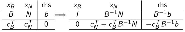
  假设我们有一个基本可行解\(\hat{\mathbf{x}} = \begin{bmatrix} \mathbf{B}^{-1} \mathbf{b} \\ \mathbf{0} \end{bmatrix}\)，\(\mathbf{A = (B, N)}\)。令\(\mathbf{x} \in \mathcal{S}\)为LP的任意一个可行解，令\(\mathbf{x} = \begin{bmatrix} \mathbf{x_B} \\ \mathbf{x_N} \end{bmatrix}\)，\(\mathbf{c} = \begin{bmatrix} \mathbf{c_B} \\ \mathbf{c_N} \end{bmatrix}\)，那么\(\mathbf{B x_B + N x_N = b}\)且\(\mathbf{x_B} = \mathbf{B}^{-1} \mathbf{b} - \mathbf{B}^{-1} \mathbf{N x_N}\)

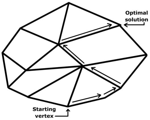
\[\begin{aligned} \mathbf{c}^T \mathbf{x} &= \mathbf{c_B}^T \mathbf{x_B} + \mathbf{c_N}^T \mathbf{x_N} \\ &= \mathbf{c_B}^T \mathbf{B}^{-1} \mathbf{b} - \mathbf{c_B}^T \mathbf{B}^{-1} \mathbf{N x_N} + \mathbf{c_N}^T \mathbf{x_N} \\ &= \mathbf{c}^T \hat{\mathbf{x}}^{T} + (\mathbf{c_N}^T - \mathbf{c_B}^T \mathbf{B}^{-1} \mathbf{N}) \mathbf{x_N} \end{aligned}\]

令\(\color{green}{r_{\mathbf{N}} = \mathbf{c_N}^T - \mathbf{c_B}^T \mathbf{B}^{-1} \mathbf{N}}\)（被称为reduced cost），如果\(r_{\mathbf{N}} \ge 0\)，那么\(\mathbf{c}^T \mathbf{x} \ge \mathbf{c}^T \hat{\mathbf{x}}^T\)并且当前的极点\(\hat{\mathbf{x}}^T\)是optimal的。否则，一定存在一个\(r_i \lt 0\)，可以令当前的非基变量\(x_i\)变成基变量\(x_i \gt 0\)（entering variable）。再选择一个合适的基变量变成非基变量（leaving variable），就可以得到一个新的基本可行解，新的解的目标函数值小于当前基本可行解\(\hat{\mathbf{x}}\)的。

  在几何学上，上述方法（单纯形法）从一个极点移动到其相邻的一个极点。由于只有有限数量的极点，该方法会在最优解处终止或者发现问题不可行的或无下界的。

• Step 0：计算初始基\(\mathbf{B}\)和基本可行解\(\mathbf{x} = \begin{bmatrix} \mathbf{B}^{-1} \mathbf{b} \\ \mathbf{0} \end{bmatrix}\)
• Step 1：如果\(r_{\mathbf{N}} = \mathbf{c_N}^T - \mathbf{c_B}^T \mathbf{B}^{-1} \mathbf{N} \ge 0\)，STOP，\(\mathbf{x}\)是一个最优解；否则，Step 2
• Step 2：选一个满足\(\mathbf{c}_j^T - \mathbf{c_b}^T \mathbf{B}^{-1} a_j \lt 0\)的\(j\)，如果\(\bar{a}_j=\mathbf{B}^{-1} \mathbf{a}_{j} \leq 0\)，STOP，该LP无界；否则，Step 3
• Step 3：计算步长\(\lambda=\min \left\{\frac{\bar{\mathbf{b}}_{i}}{\bar{\mathbf{a}}_{i j}} \mid \bar{\mathbf{a}}_{i j} \gt 0\right\}=\frac{\bar{\mathbf{b}}_{r}}{\bar{\mathbf{a}}_{r j}} \ge 0\)，令\(\mathbf{x} := \mathbf{x} + \lambda \mathbf{d}_j\)，其中\(\mathbf{d}_j = \begin{bmatrix} \mathbf{B}^{-1} \mathbf{a}_j \\ \mathbf{e}_j \end{bmatrix}\)，返回Step 1。

1.1.3 Duality

Dual theory: motivation

  考虑如下单一等式约束的最小化问题：

\[\text{(P)} \quad \begin{array}{ll} \min & f(x) \\ \text {s.t.} & h(x)=0 \\ & x \in X \end{array}\]

其中，\(h(x)=0\)是一个hard constraint，\(x \in X\)是一个easy constraint。

这个问题该怎么解决呢？

• 有一个想法，通过放松硬约束\(h(x)=0\)来解决一个更简单的问题。
• 这可以通过将约束纳入目标函数来实现。如果违反了约束，就会带来相应的price。

  给定一个Lagrangian multiplier \(\color{green}{\lambda}\)（price），那么Lagrangian dual function定义为

\[d(\lambda) = \min _{x \in X} L(x, \lambda) := f(x)+\lambda h(x)\]

给出了(P)的lower bound：

\[d(\lambda) \le f(x), \forall \text{ feasible solution of (P)}\]

  最优下界可以通过解\(\text{(D)} \ \max_{\lambda} d(\lambda)\)得到，(D)被称为(P)的Lagrangian dual problem。

Dual of LP

  考虑标准LP：

\[\text{(P)} \quad \begin{array}{ll} \min & \mathbf{c}^T \mathbf{x} \\ \text {s.t.} & \mathbf{Ax = b}, \mathbf{x} \ge 0 \end{array}\]

将乘数\(\pmb{\lambda} \in \mathbb{R}^m\)与\(\mathbf{Ax = b}\)联系起来，得到dual funtion

\[d(\pmb{\lambda}) = \min_{x \geq 0} {\mathbf{c}^T \mathbf{x} + \pmb{\lambda}^{T}(\mathbf{b-A x})} = \mathbf{b}^{T} \pmb{\lambda} + \min_{x \geq 0}(\mathbf{c} - \mathbf{A}^{T} \pmb{\lambda})^{T} \mathbf{x} = \begin{cases} \mathbf{b}^{T} \pmb{\lambda}, & \text { if } \mathbf{A}^{T} \pmb{\lambda} \leq \mathbf{c} \\ -\infty, & \text { otherwise } \end{cases}\]

所以，对偶问题为

\[\text{(D)} \quad \begin{array}{ll} \max & \mathbf{b}^T \pmb{\lambda} \\ \text {s.t.} & \mathbf{A}^{T} \pmb{\lambda} \le \mathbf{c} \end{array}\]

Inequality constraints

  考虑LP：

\[\text{(P)} \quad \begin{array}{ll} \min & \mathbf{c}^T \mathbf{x} \\ \text {s.t.} & \mathbf{Ax \ge b} \\ & \mathbf{x} \ge 0 \end{array}\]

添加松弛变量\(\mathbf{s} \ge 0\)，得到\(\begin{bmatrix} \mathbf{A} & -\mathbf{I} \end{bmatrix} \begin{bmatrix} \mathbf{x} \\ \mathbf{s} \\ \end{bmatrix} = \mathbf{b}\)，这会带来对偶约束\(\begin{bmatrix} \mathbf{A} & -\mathbf{I} \end{bmatrix}^T \pmb{\lambda} = \le \begin{bmatrix} \mathbf{c} \\ \mathbf{0} \\ \end{bmatrix} = \mathbf{b}\)。
因此，LP的对偶问题为

\[\text{(D)} \quad \begin{array}{ll} \max & \mathbf{b}^T \pmb{\lambda} \\ \text {s.t.} & \mathbf{A}^{T} \pmb{\lambda} \le \mathbf{c} \\ \pmb{\lambda} \ge \mathbf{0} \end{array}\]

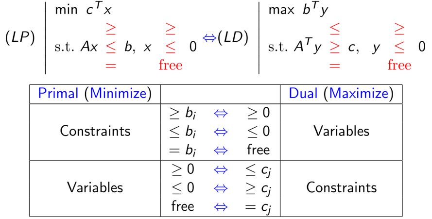
Primal & Dual forms

我们可以将一般LP对偶如下:

1.2 Branch-and-bound method

分支定界策略：

• 求解问题的线性松弛。如果解是整数，那么就做完了。否则，通过在一个分数解发展分支来构造两个子问题。
• 当以下任一情况发生时，一个节点（子问题）是不活跃的:
   （1）节点正在被分支；
   （2）解是整数；
   （3）子问题不可行；
   （4）你可以通过一个边界参数来理解子问题。
• 选择一个活跃节点并在分数变量处分支。重复以上过程直到不存在活跃的子问题。

这是一个部分枚举的过程，所以分支定界法也称partial enumeration.

例：考虑如下0-1背包问题：

\[\begin{array}{ll} \max & 8 x_{1}+11 x_{2}+6 x_{3}+4 x_{4} \\ \text { s.t. } & 5 x_{1}+7 x_{2}+4 x_{3}+3 x_{4} \leq 14 \\ & x \in\{0,1\}^{4} \end{array}\]

其线性松弛问题的解为\(\mathbf{x} = (1, 1, 0.5, 0)\)，对应的值为22，这个解是非整数的。选择\(x_3\)来发展分支，那么两个子问题就分别是\(x_3 = 0\)和\(x_3 = 1\)。
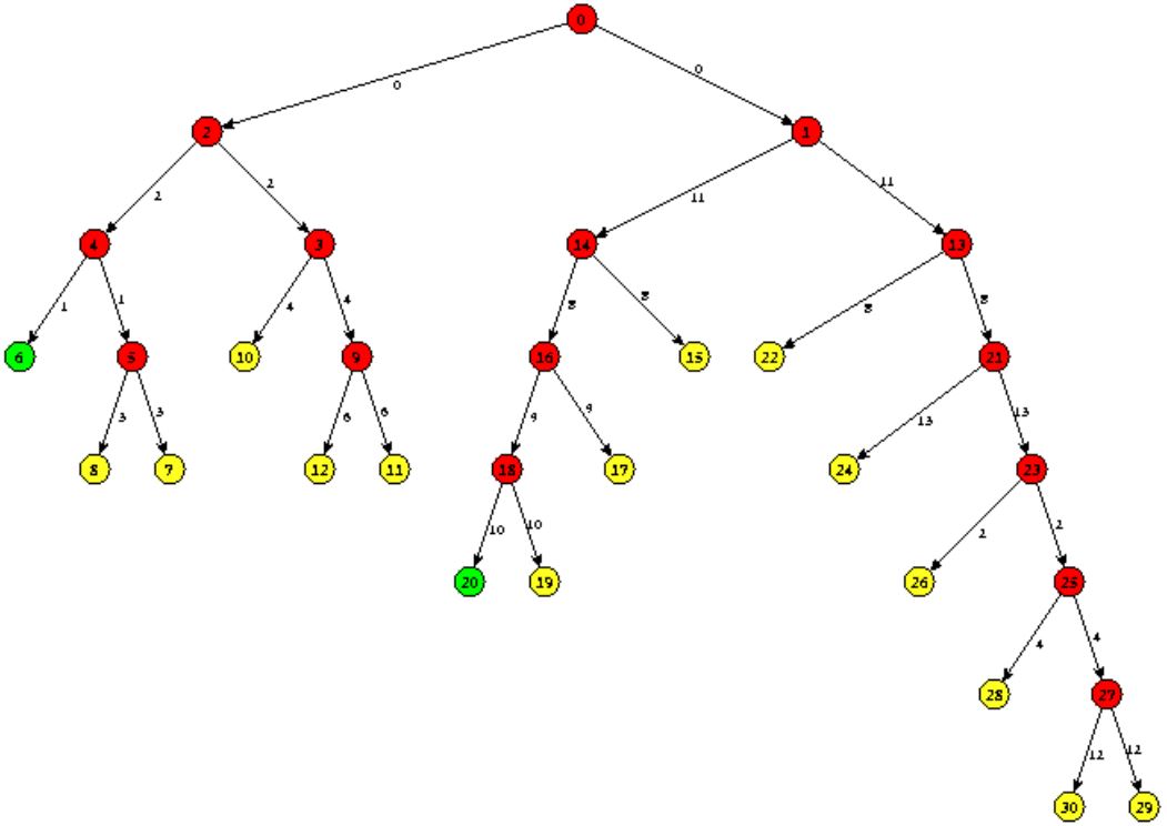
搜索树为：

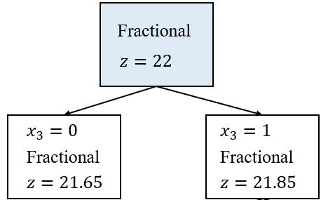
这两个子问题的线性松弛解为
  \(x_3 = 0\)：\(\mathbf{x} = (1, 1, 0, 0.667)\)，目标值\(= 21.65\)
  \(x_3 = 1\)：\(\mathbf{x} = (1, 0.714, 1, 0)\)，目标值\(= 21.85\)。
此时可以知道最优值不会比21.85多（实际上，我们知道最优值应该小于或等于21。）但是，我们仍然没有得到任何可行的整数解，所以我们选择一个子问题并在它的某一个变量发展分支。

选\(x_3 = 1\)为节点，按\(x_2\)分支，对应的搜索树为：

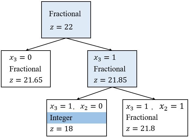
线性松弛解为
  \(x_3 = 1, x_2 = 0\)：\(\mathbf{x} = (1, 1, 1, 1)\)，目标值\(= 18\)
  \(x_3 = 1, x_2 = 1\)：\(\mathbf{x} = (0.6, 1, 1, 0)\)，目标值\(= 21.8\)。

选\(x_3 = 1, x_2 = 0\)为节点，按\(x_1\)分支，对应的搜索树为：

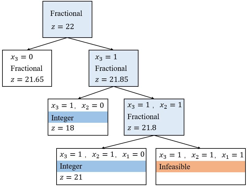
线性松弛解为
  \(x_3 = 1, x_2 = 0, x_1 = 0\)：\(\mathbf{x} = (0, 1, 1, 1)\)，目标值\(= 18\)
  \(x_3 = 1, x_2 = 1, x_1 = 1\)：不可行。

  最优解为\(\mathbf{x} = (0, 1, 1, 1)\)。

1.2.1 0-1 Knapsack by B&B

\[\text{(0-1 KP)} \quad \max \{ \mathbf{c^T x} \mid \mathbf{a^T x \le b}, \mathbf{x} \in \{0, 1\}^n \}\]

  要解(0-1 KP)的LP松弛问题，只需要用贪心算法！假设变量的顺序为\(c_1 / a_1 \ge c_2 / a_2 \ge \cdots \ge c_n / a_n\)，令\(s\)为取到最大时的序号\(k\)，则\(\sum_{j=1}^k a_j \le b\)。

Theorem (Dantzig, 1957)：(0-1 KP) 的连续松弛问题的最优解为

\[\begin{aligned} &w_j=1, j=1, \ldots, s, \\ &w_j=0, j=s+2, \ldots, N, \\ &w_{s+1}=\left(b-\sum_{j=1}^s a_j\right) / a_{s+1} . \end{aligned}\]

如果\(c_j, j = 1, \ldots, N\)是正整数，那么(LKP)最优值的上界为

\[\text{UB} = \sum_{j=1}^s c_j + \left\lfloor(b-\sum_{j=1}^s a_j) c_{s+1} / a_{s+1}\right\rfloor\]

1.2.2 How to branch?

  我们想把当前的问题分成两个或更多的子问题，让它们比原来的问题更容易。一个常用的分支方法是：

\[x_i \le \left\lfloor x_i^* \right\rfloor, x_i \ge \left\lceil x_i^* \right\rceil\]

其中，\(x_i^*\)是一个分数变量。

  选哪个变量来分支呢？一个常用的分支规则是：branch the most fractional variable，即在离整数点最远的变量处分支。

  我们希望能够选择一个分支能让解决所有子问题所花的时间最短。我们要如何知道解每个子问题所需的时间呢？答案是不能，但是我们有一个idea：尝试预测子问题的困难程度。

  一个比较好的分支规则：线性规划的松弛值改变了很多!

1.2.3 Which node to select?

  分支定界法中的一个重要选择是选择下一个要处理的子问题的策略。目标：（1）最小化总的求解时间；（2）快速找到一个好的可行的解决方案。

一些常用的搜索策略：

• Best First
• Depth-First
• Hybrid Strategies
• Best Estimate

The best first approach

  最小化总求解时间的一种方法是尽量最小化搜索树的大小。我们可以通过选择具有最优上界的子问题来实现这一点(最小化时的下界是最低的)。

最佳优先搜索的缺点：

• 不一定能很快找到可行的解决方案，因为可行的解决方案"更有可能"在树的深处找到
• 节点设置成本很高。所求解的线性规划在每次计算节点时可能会有很大的变化
• 内存占用率过高。它可能需要大量内存来存储候选列表，因为树可能长得很"宽"

The deap First approach

  深度优先的方法总是选择最深的节点进行下一步处理。只要一直往下，直到你需要剪枝，然后返回走另一条路。这避免了最佳优先搜索的大多数问题：最小化候选节点的数量（节省内存）和节点设置成本最小化。LPs从一个迭代到下一个迭代变化很小，通常很快就能找到可行的解决方案。

  缺点：如果初始下界不是很好，那么我们最终可能会处理很多非关键节点。

  混合策略：先进行深度优先搜索直到你找到一个可行的解决方案，然后做最佳优先搜索。

1.3 Software for integer programming

Matlab code: bintprog可以解决0-1整数线性规划问题

商业优化软件CPLEX和Gurobi可以解决混合整数线性和二次规划问题。
调用CPLEX MIP求解器的两种简单方法:
 1. Optimization Programming Language (OPL) in CPLEX Optimization Studio.
 2. CPLEX Matlab interface.